|
|
Non-Uniform Sampling (NUS) in NMRPipe Conversion of NUS DataReconstruction of NUS Data via NMRPipe's Iterative Shrinkage Thresholding (IST) Using IST on Conventional Data as an Alternative to Linear Prediction See Also: Using Non-Uniformly Sampled Data in NMRPipe (NMRPipe_NUS_v44.pptx 20MB) |
Non-Uniform Sampling (NUS) is an acquisition method for multidimensional NMR spectra that works by skipping some fraction of the data that would be acquired in a conventional measurement, which is uniformly sampled (US). The goal of NUS is to improve the spectral resolution (or possibly other metric of spectral quality) obtained with a given amount of measurement time.
Because some of the data is skipped in a NUS acquisition, the usual Fourier transform processing used for conventional data is not ideal, and so other reconstruction methods are required to take best advantage of NUS.
There are many tools from other labs for reconstructing NUS data, including Matrix Decomposition (MDDNMR software), Maximum Entropy (The Rowland NMR Toolkit), Iterative Soft Thresholding (IST) (hmsIST software), SCRUB, and NESTA. Many of these tools use NMRPipe as part of the reconstruction workflow, and they will often have schemes for converting NUS data that are different from the ones discussed here.
NMRPipe includes its own implementation of IST, so that it is easy to perform all the steps needed for NUS reconstruction. This document and corresponding demo data shows how to use NMRPipe to convert NUS NMR data, and how to reconstruct NUS spectra using NMRPipe's implementation of IST. NMRPipe's implementation of IST will only yield good results when indirect dimensions have first order phase corrections P1 of 0, 180, or 360.
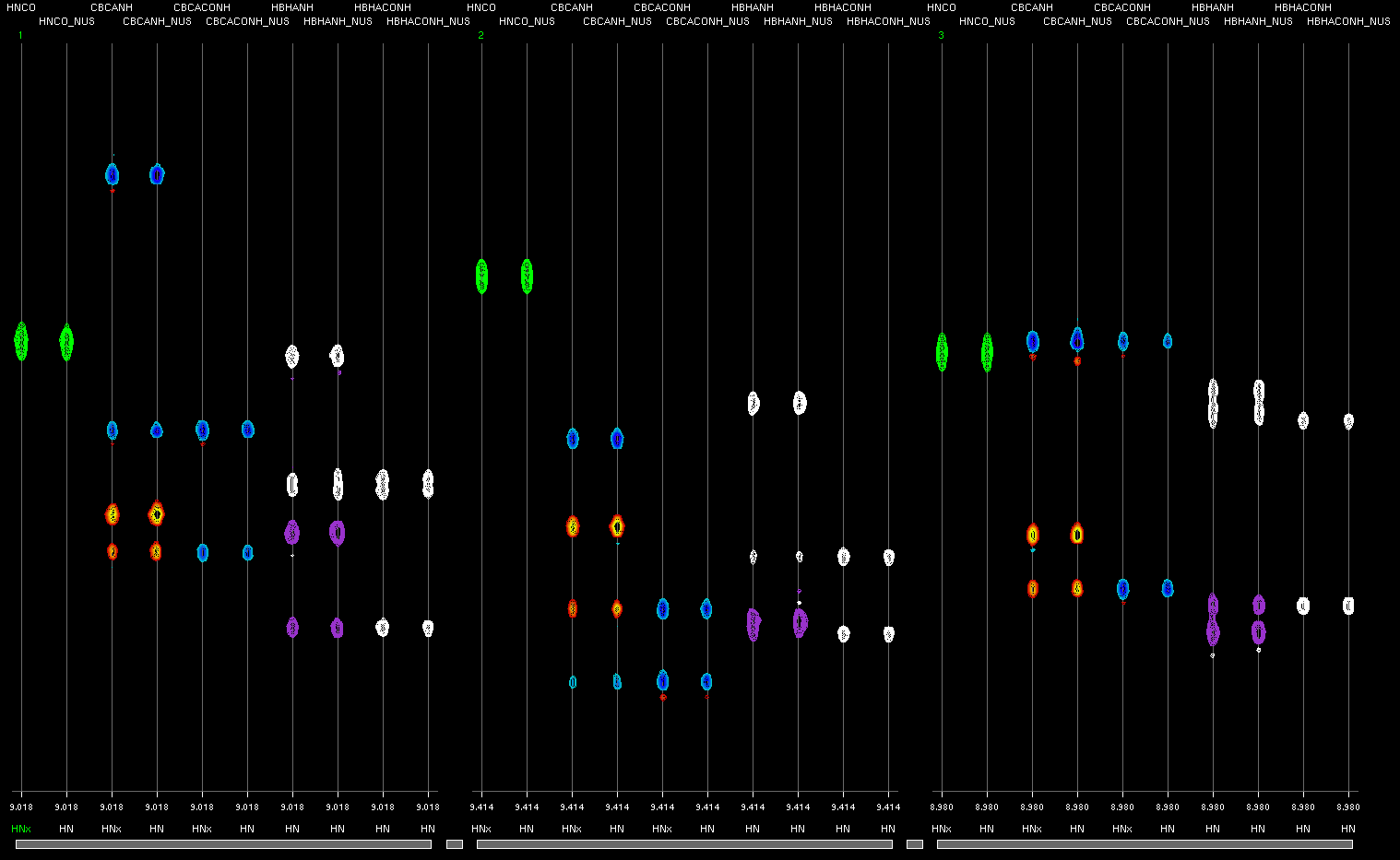
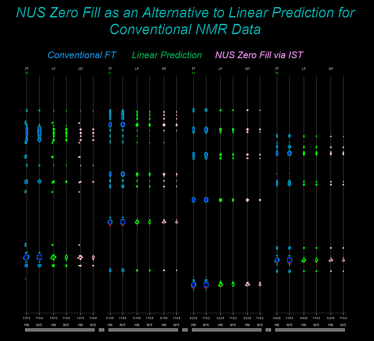
As noted by Hoch et al., since IST can be thought of as a method for reducing Fourier reconstruction artifacts, it can also be applied to conventional data as an alternative to Linear Prediction (Hoch et al. 2007 below). We call this method NUS Zero Fill, and the conventional spectra in the demo data include examples of this method as well.
The NMRPipe Demo Data collection includes NUS examples kindly provided by Robert Brinson and Luke Arbogast at IBBR, Jinfa Ying at the NIH, Prof. Stefano Ciurli at the University of Bologna, and Massimo Lucci at the University of Florence. The details of the NUS demo data are provided at the end of this document.
Some Related References
A.S. Stern, D.L. Donoho, and J.C. Hoch: NMR data processing using iterative thresholding and minimum l(1)-norm reconstruction. J Magn Reson., 188, 295-300 (2007).
S.G. Hyberts, K. Takeuchi, and G. Wagner: Poisson-gap sampling and forward maximum entropy reconstruction for enhancing the resolution and sensitivity of protein NMR data. J Am Chem Soc., 132, 2145-2147 (2010).
V. Orekhov and V. A. Jaravine: Analysis of non-uniformly sampled spectra with Multi-Dimensional Decomposition. Progress in Nuclear Magnetic Resonance Spectroscopy, 59, 271-292 (2011).
B.E. Coggins, J.W. Werner-Allen, A. Yan, and P. Zhou: Rapid Protein Global Fold Determination Using Ultrasparse Sampling, High-Dynamic Range Artifact Suppression, and Time-Shared NOESY. J. Am. Chem. Soc., 134, 18619-18630 (2012).
K. Kazimierczuk and V. Orekhov: A comparison of convex and non-convex compressed sensing applied to multidimensional NMR. J Magn Reson., 223, 1-10 (2012).
S.G. Hyberts, A.G. Milbradt, A.B. Wagner, H. Arthanari, and G. Wagner: Application of iterative soft thresholding for fast reconstruction of NMR data non-uniformly sampled with multidimensional Poisson Gap scheduling. J Biomol NMR., 52, 315-27 (2012).
S.G. Hyberts, H. Arthanari, S.A. Robson, and G. Wagner: Perspectives in magnetic resonance: NMR in the post-FFT era. J Magn Reson., 241, 60-73 (2014).
J.C. Hoch, M.W. Maciejewski, M. Mobli, A.D. Schuyler, and A.S. Stern: Nonuniform sampling and maximum entropy reconstruction in multidimensional NMR. Acc Chem Res., 47, 708-17 (2014).
S. Sun, M. Gill, Y. Li, M. Huang, and R.A. Byrd: Efficient and generalized processing of multidimensional NUS NMR data: the NESTA algorithm and comparison of regularization terms. J Biomol NMR., 62, 105-117 (2015).
A.S. Stern and J.C. Hoch: A new approach to compressed sensing for NMR. Magn Reson Chem., 53, 908-912 (2015).
About Non-Uniform Sampling
In a conventional 2D experiment, the indirect dimension is uniformly sampled, or more specifically, it is acquired as a series of 1D measurements at N uniformly-spaced time increments in increasing order:
time coordinate of measurement k = k*dT + delay
where dT is the time increment, delay is the initial acquisition delay,
and k is the increment number which goes from 0 to N - 1.
As a general rule, spectral width will be proportional to 1/dT,
and resolution will be inversely proportional to the largest time
coordinate acquired (that is, the greater the largest time, the
better the resolution). As a side note, the delay will often be one of three cases:
    delay = 0     (first order phase correction P1 = 0)
    delay = dT/2  (first order phase correction P1 = 180)
    delay = dT    (first order phase correction P1 = 360)
Given the description above, we can represent the measurement scheme for an indirect dimension of an NMR measurement as a list of values for the increment number, k. For a conventional linearly-sampled data set with 16 indirect points (N = 16), the sampling schedule would simply be:
    0
    1
    2
    3
    4
    5
    6
    7
    8
    9
   10
   11
   12
   13
   14
   15
In a NUS scheme, one or more increments are skipped (not measured at all) during the acquisition. Choosing which increments to skip might be done randomly, or according to some mathematical function. Whatever method is used, the NUS schedule can still be represented by a list of increment numbers, and these will be a subset of the numbers in the linearly-sampled schedule. For example, a NUS version of the linear schedule above could randomly skip half of the increments, as shown here:
    0
    1
    3
    5
    8
   10
   11
   15
As noted, resolution will be inversely proportional to the largest time
coordinate acquired (that is, the greater the largest time, the
better the resolution). In both the linear and NUS schedule above,
the largest time value is the same, for k = 15. So, both schedules
represent data of the same spectral width and resolution. But, since
the NUS schedule has half the number of increments, if all other
details are the same (such as number of scans per increment), it will take half
the amount of actual instrument time to measure the NUS data. It is
important to note though, that by decreasing the number of increments
measured, the signal-to-noise will also be reduced.
In some NUS schemes, the increments are measured in random order. One advantage of this is that an experiment can be stopped before all increments have been measured, and the resulting data can still span larger time values and hence have better resolution. For example, if the NUS schedule above was stopped after 5 of the 8 increments had been measured, the resolution would correspond to the largest k value, which in the NUS schedule above would be k = 8. But for the example random-order NUS schedule which follows, the resolution would correspond to the largest k value in the first 5 increments, which in this case is k = 11:
    0
    1
   11
    5
    8
    3
   15
   10
As described, the NUS schedule for 2D data can be represented by a text file of increment numbers like the examples above, with one integer value per line. Depending on the convention used to measure the data, the increment numbers might start at 1, instead of at 0 as in the examples above.
In the case of 3D data, the NUS schedule will have two values per line, one corresponding to a time increment in the Y-Axis, and the other corresponding to a time increment in the Z-Axis. The order that these two values are given on a line depends on the convention used to measure the data. Similarly, NUS schedules for 4D data will have three values per line, for the Y-Axis, Z-Axis, and A-Axis, and the order that these are given on a line can also vary.
How NMRPipe Handles NUS Data
In NMRPipe NUS schemes, the sampling schedule text files described above are used as input to reorder and expand the data. This is is usually done in one of two ways:
- The raw spectrometer format data, regardless of the number of dimensions, is converted without change as an NMRPipe-format 2D time-domain data set. It is then reordered and expanded in later steps, often after NMRPipe has been used to process the directly-detected dimension of the data.
- The raw spectrometer format data is directly reordered and expanded with zeros to generate a new copy of the raw data, which can then be converted and processed with the same schemes that would be used for conventional data.
All of the demo examples here use approach (2) above, because it tends to result in simpler and more consistent conversion and processing schemes, and it allows the NUS data to be processed by conventional Fourier transform and inspected before more time-consuming reconstruction is applied.
The NMRPipe NUS expansion tools also create NMRPipe-format data files which encode the sampling schedule as ones and zeros, and these are used as additional input for NMRPipe's own NUS reconstruction tools. Two kinds of NMRPipe-format data are created, called the kernel, and the mask.
The mask corresponds directly to the time-domain data; it is identical
in size to the expanded time-domain data, but it is set to 1.0 for every
point in the data that was measured in the NUS schedule, and 0.0 for
every point that was skipped. The mask is used as input for NMRPipe's
Iterative Shrinkage Thresholding (IST) Reconstruction. By default,
the mask is named mask.fid for 2D data,
and mask/test%03d.fid for 3D data.
The kernel file corresponds to only the indirect dimensions
involved in the NUS schedule. So, for example, if 2D NUS data is expanded
into 2D time-domain data with 32 points in the indirect dimension,
then the kernel will be a 1D NMRPipe-format data with 32 points.
This kernel data will be set to 1.0 at every position where an
increment was measured, and 0.0 at every position where an increment
was skipped. This file can be used as input for NMRPipe's Maximum
Entropy deconvolution or Maximum Likelihood analysis, although these
are not illustrated here. By default, the kernel files are named
profY.dat for 2D data, and profYZ.dat for 3D.
About NMRPipe's Iterative Shrinkage Thresholding (IST) Reconstruction
In a conventional multidimensional NMR experiment, the indirect dimensions are sampled with uniform time increments, and reconstructed by Fourier transform. In a NUS experiment, some fraction of these samples are skipped. As explained above, the pattern of which samples are measured and which are skipped is called the sampling schedule. Because of the missing data, an ordinary Fourier transform will have artifact bands according to the pattern of samples that have been skipped. The shape of the artifacts is the same for every peak, and the size of the artifacts is proportional to the height of the peaks.
Since the ordinary Fourier transform of NUS data will not give an ideal result, other methods are used to generate a spectrum. The examples here use NMRPipe's implementation of IST, which takes expanded time-domain data and a corresponding mask as input, and produces a reconstructed spectrum as output. NMRPipe's IST also requires specification of accurate phase correction values to work properly.
The IST reconstruction is iterative. It takes advantage of the fact that the NUS artifacts are proportional to the size of the peaks. In the course of an IST reconstruction, intensity is gradually moved from the tops of the highest remaining signals, and the intensity that was removed is accumulated in a reconstruction. As the signals are reduced, the artifacts are reduced as well.
The NMRPipe implementation of IST has three main adjustable parameters:
| Parameter | Default Value | Common Range | Description |
|---|---|---|---|
| istMaxRes | 1.0 | 0.1 to 1.0 | A percentage defining the condition for convergence. |
| istTMult | 0.7 | 0.7 to 0.9 | A fraction specifying the threshold for intensity reduction. Rarely changed, should usually not be set less than 0.7. |
| istCMult | 0.3 | 0.1 to 0.9 | A fraction specifying the amount of intensity reduction above the threshold. Rarely changed. |
An Important Limitation of NMRPipe's IST Reconstruction
NMRPipe's implementation of IST uses a Hilbert transform to reconstruct imaginary data at each iteration. The Hilbert transform is only exact for cases where the first-order phase P1 is zero or a multiple of 180. Other first-order phase corrections yield baseline distortions. As a result, NMRPipe's implementation of IST will only yield good results when the indirect dimensions have first order phase corrections P1 of 0, 180, or 360.
NMRPipe's IST Algorithm
The NMRPipe implementation of IST works as follows:
-
Start with NUS time-domain data
T, which has been sorted and expanded to correspond to uniformly sampled data, but with the parts that were skipped in the NUS sampling schedule set to zero. Apply a complete Fourier processing scheme with window functions and phase correction to generate initial spectrumF, which has the imaginary parts deleted during processing. -
Inverse process the indirect dimensions of spectrum
Fto produce interferogramD. During inverse processing, imaginary data is reconstructed by Hilbert transform, and any phase correction that was applied during forward processing is removed. -
Set the parts of interferogram
Dthat were skipped in the sampling schedule to zero. -
Fourier transform and phase correct the indirect dimensions of
interferogram
Dto generate a new version of spectrumF, which has the imaginary parts deleted during processing. No window functions are applied. -
Find
maxVal, the maximum value of the spectrumFat this iteration. If this is the first iteration, save this value asmaxValFirst. -
Choose a threshold "thresh" for reducing the intensities in spectrum
Fat this iteration:thresh = istTMult*maxValNothing below this threshold is changed during this iteration. The data above this threshold is scaled down by
istCMult, so that each current value in spectrumFwhich is above the threshold is replaced by a new value:new F value = istCMult*(current F value - thresh) + thresh -
Correspondingly, update each value in NUS reconstruction
Sby adding the intensity that was removed from spectrumF:new S value = current S value + current F value - new F value -
Repeat steps 2 to 7 until convergence, where the maximum value of the
remaining residual in
Fis below the specified target. The target is specified as a percentage of the maximum value in the first-iteration spectrum:convergence when maxVal < istMaxRes*maxValFirst/100.0 -
After convergence, a zero-order baseline correction is applied to the remaining
residual in
F, and the result is added to the final NUS reconstructionS. - If any post-reconstruction baseline corrections were specified, these are applied to the final NUS reconstruction.
Usual Steps for Converting and Processing NUS Data in NMRPipe
Non-Uniform Sampling (NUS) works by skipping parts of the measurement that would be acquired in a conventional experiment. The pattern of parts that are kept or skipped is called the sampling schedule.
The general steps in a usual workflow for reconstructing NUS data with NMRPipe are as follows:
- Build and execute a conversion script which sorts and expands the NUS data from the spectrometer to generate NMRPipe-format time-domain data. At this point, the NUS data has zeros in the parts of the measurement that were skipped.
- Confirm processing parameters such as phase correction by performing conventional processing with the usual NMRPipe facilities.
- Use the processing parameters to run NMRPipe's NUS reconstruction scripts.
The steps in more detail follow:
-
Build a conversion script by starting the usual NMRPipe format
conversion interface, using the
-nusoption to enable features for NUS. So, depending on the source of data, the command will be:bruker -nusorvarian -nus - Use the graphical interface to set Spectrometer Input as usual, and also select the NUS Schedule, the text file input containing the NUS sampling schedule.
-
Use Read Parameters and then interactively adjust the conversion
parameters as usual. Set the NUS-related parameters appropriately:
- NUS Samples: the number of NUS increments that were actually measured. When keyword Auto is specified, this will be set to the number of samples found in the NUS schedule file. Set it to a smaller number for measurements that were stopped before they were complete.
- NUS Index Offsets: the index offset is the number to be subtracted from the increment numbers in the NUS schedule file input, so that the result matches the NMRPipe convention of having the first increment number as zero. It is intended to account for the whether the increment numbers in the input file start with 0 or 1, and as such, it is usually set to 0 or 1. When keyword Auto is specified, it will be set to the smallest number found in the NUS schedule file. In most cases, only a single value needs to be specified, and the same value will be used for all increment numbers in the schedule. In certain advanced applications, a list of numbers, one for each indirect dimension, can be specified.
- Reverse NUS Column Order accounts for the order that increment values are given on each line of a 3D or 4D NUS schedule. By default, each line is expected to start with the increment number for the Y-Axis. Turn this checkbox on if the NUS schedule file lines give the increments in opposite order, with the Y-Axis increment last on each line.
-
When the parameters have been adjusted as needed, use Save Script
to save the conversion script. The graphical interface will create
a conversion script with these steps:
-
Using the sampling schedule information, sort and expand
the spectrometer input so that the missing samples are
filled in with zeros. This is done via the script
nusExpand.tcl, or for older NUS formats, by the scriptvdExpand.tcl -
Convert the expanded data as usual via
bruk2pipeorvar2pipe. -
Use the converted data to build an NMRPipe-format mask, also
done via the script
nusExpand.tcl. This mask will be the same size as the converted data, but consist of only ones and zeros according to which parts of the measurement were skipped in the sampling schedule. The mask is used as input for later reconstruction steps.
bruker -nus:#!/bin/csh nusExpand.tcl -mode bruker -sampleCount 2048 -off 0 \ -in ./ser -out ./ser_full -sample ./nuslist bruk2pipe -in ./ser_full \ -bad 0.0 -aswap -AMX -decim 1680 -dspfvs 20 -grpdly 67.9866027832031 \ -xN 2048 -yN 64 -zN 320 \ -xT 1024 -yT 32 -zT 160 \ -xMODE DQD -yMODE Echo-AntiEcho -zMODE Complex \ -xSW 11904.762 -ySW 3846.154 -zSW 11904.762 \ -xOBS 950.204 -yOBS 96.294 -zOBS 950.204 \ -xCAR 4.773 -yCAR 118.579 -zCAR 4.773 \ -xLAB HN -yLAB 15N -zLAB 1H \ -ndim 3 -aq2D States \ -out ./fid/test%03d.fid -verb -ov xyz2pipe -in ./fid/test%03d.fid \ | nusExpand.tcl -mask -noexpand -mode pipe -sampleCount 2048 -off 0 \ -in stdin -out ./mask/test%03d.fid -sample ./nuslist -
Using the sampling schedule information, sort and expand
the spectrometer input so that the missing samples are
filled in with zeros. This is done via the script
-
The NUS conversion script displays a substantial amount of informational
text, so it is best executed from the command line rather than
via the Execute Script button in the conversion interface. So, use Quit to
exit the conversion interface, and execute the conversion script
from the UNIX command-line:
fid.com -
After executing the conversion script, first try ordinary Fourier
processing of the expanded NUS data. In the case of 3D data, generate
and inspect 2D projections of the processed result using the
proj3D.tclcommand. If 3D data is expected to have a combination of positive and negative signals, use absolute-value projectionproj3D.tcl -abs ...In order to simplify this trial processing of the NUS data, there are two general-purpose scripts
basicFT2.comandbasicFT3.comwhich can perform complete processing schemes using parameters from the command-line. TrybasicFT2.com -helpandbasicFT3.com -helpfor more details. ThebasicFT2.comscript can perform 2D processing on 2D data, or extract and process a 2D XY or XZ plane from 3D data.The scripts automatically set first-point scaling based on phase correction values, and for HN-detected data, they add solvent correction and baseline correction by default. So in practice, complete processing can be specified with just a small number of parameters, primarily by specifying any non-zero phase correction parameters and the region of interest to extract. For example, these commands will process the first XY plane and XZ plane of a 3D, process the complete 3D, and create 2D projections of the 3D result:
basicFT2.com -xy -in fid/test%03d.fid -out xy.ft2 \ -xP0 13 -xP1 0 -xEXTX1 10.4ppm -xEXTXN 5.4ppm \ -yP0 -90 -yP1 180 basicFT2.com -xz -in fid/test%03d.fid -out xz.ft2 \ -xP0 13 -xP1 0 -xEXTX1 10.4ppm -xEXTXN 5.4ppm \ -yP0 0 -yP1 0 \ -yFTARG alt basicFT3.com -in fid/test%03d.fid -out ft/test%03d.ft3 \ -xP0 13 -xP1 0 -xEXTX1 10.4ppm -xEXTXN 5.4ppm \ -yP0 -90 -yP1 180 \ -zFTARG alt proj3D.tcl -in ft/test%03d.ft3 -abs -
Inspect the conventionally-processed data and projections. This will
usually help to confirm that conversion was performed properly,
and that phase correction and Fourier transform options are set
properly. Things to look for:
-
Dimension has a mirror image: as with conventional data, this
will happen if
-yMODEor-zMODEwere not set correctly during conversion. It will also happen if the NUS expansion step was not done properly. As noted previously, there are several possible schemes for specifying an sampling schedule and organizing NUS data during acquisition, so the schemes used for the demo data here might not be suitable for every type of NUS measurement. -
Dimension is reversed: FT
negoption is needed. -
Dimension is left-right swapped: FT
altoption is needed.
-
Dimension has a mirror image: as with conventional data, this
will happen if
-
After processing parameters have been selected and confirmed by
conventional Fourier transform, use these parameters to perform
an Iterative Shrinkage Thresholding (IST) reconstruction, via
the scripts
ist2D.comorist3D.comfor 2D or 3D data, respectively. These IST scripts have similar arguments asbasicFT2.comandbasicFT3.com, so that they can all be conveniently used together. The IST scripts take time-domain data as input, and produce a fully-processed spectrum as output. Here is an example 3D usage, with generation of 2D projections of the result:ist3D.com \ -in fid/test%03d.fid -mask mask/test%03d.fid -out ist/test%03d.ft3 \ -xP0 13 -xP1 0 -xEXTX1 10.4ppm -xEXTXN 5.4ppm \ -yP0 -90 -yP1 180 \ -zFTARG alt proj3D.tcl -in ist/test%03d.ft3 -abs -
Inspect the IST result.
If needed, repeat the IST processing with different parameter
settings, such as the IST convergence value
istMaxRes.
Estimating the Convergence Parameter istMaxRes for NMRPipe's IST
A practical choice for convergence is to stop the IST iterations when the expected sampling
schedule artifacts for the largest remaining signals would be about the same size as the
random noise in the spectrum. We can estimate this convergence value from the ordinary
Fourier transform before performing the IST calculation. The specStat.com utility can be used
to form the estimate automatically. Note that in practice, it might be necessary to adjust
this value to get a good reconstruction.
Perform ordinary Fourier processing of the expanded NUS data:
   basicFT3.com -in fid/test%03d.fid -out ft/test%03d.ft3 \
                -xP0 -75 -xP1 0 -xEXTX1 10.4ppm -xEXTXN 5.4ppm \
                -zFTARG alt
Use specStat.com to estimate the convergence parameter:
specStat.com -in ft/test%03d.ft3 -stat istMaxRes
The specStat.com utility will print a result such as:
istMaxRes 0.32451416
The istMaxRes value is calculated from an automated estimate of the noise relative to
the largest absolute value intensity in the spectrum:
istMaxRes = 3.0*100.0*vNoiseEst/vMaxAbs
NUS Zero Fill: Using IST on Conventional Data as Alternative to Linear Prediction
IST can be thought of as a method to form a reconstruction without the Fourier transform artifacts associated with a particular sampling schedule. This concept holds for both Non-Uniform and conventional Uniformly Sampled schedules. As noted by Hoch and coworkers, this means it is possible to apply IST to conventional data, as an alternative to extending data via Linear Prediction. We call this approach NUS Zero Fill.
In the NUS Zero Fill approach, we use the nusZF.com utility to take
conventional Uniformly Sampled time-domain data, zero fill it in the indirect dimensions,
and build a "synthetic" sampling schedule and mask to describe the uniformly sampled
zero-filled result.
So, in the same way as for a NUS scheme, as an initial step we can process the data
with an ordinary Fourier transform, and use the transformed spectrum to
estimate the istMaxRes convergence parameter. Then we can use the
utility nusZF.com to prepare the zero-filled data and mask, and use these as input for IST:
      % basicFT3.com -in fid/test%03d.fid -out ft/test%03d.ft3 \
         -xP0 -201.1 -xP1 0.0 -xEXTX1 10.0ppm -xEXTXN 5.5ppm \
         -yP0   45.0 -yP1 0.0

      % specStat.com -in ft/test%03d.ft3 -stat istMaxRes

      istMaxRes 0.10764479

      % nusZF.com -in fid/test%03d.fid \
         -out nuszf/test%03d.fid -mask mask/test%03d.fid

      % ist3D.com -istMaxRes 0.11 \
         -in   nuszf/test%03d.fid -mask mask/test%03d.fid -out ist/test%03d.ft3 \
         -xP0 -201.1 -xP1 0.0 -xEXTX1 10.0ppm -xEXTXN 5.5ppm \
         -yP0   45.0 -yP1 0.0 -xBASEARG POLY,auto
There are two important comments about using NMRPipe's IST in NUS Zero Fill schemes:
-
Larger Convergence Parameter: Sampling schedule reconstruction artifacts in conventional
data (i.e., truncation wiggles) are usually no more than 20% as large as their corresponding signals,
and often much less. By contrast, NUS artifacts can be 40% or more as large as their corresponding signals.
So, it may be appropriate to use larger values of
istMaxResfor NUS Zero Fill applications, since these will not need as much artifact reduction as similar NUS cases. -
Specify Baseline Correction:If baseline correction is appropriate (as is usual for HN-detected spectra)
it should be specified explicitly when using IST for NUS Zero Fill
(
xBASEARG POLY,autoabove). This will perform baseline correction on the starting spectrum, before IST reconstruction begins. By default, IST defers baseline correction until after the IST reconstruction is complete (-xBASEARG_FINAL). This is a compromise for NUS data, where it is difficult perform baseline correction effectively before reconstruction.
Tips for NUS Reconstruction with NMRPipe's IST
Baseline distortion is especially problematic for NUS reconstruction, because it is difficult to correct baseline effectively before or during the reconstruction.
Likewise, interactive phasing of the indirect dimensions can be difficult, because prior knowledge of the phase correction values is required for a good IST reconstruction.
- As a general point for either conventional or NUS measurement, take care to set initial delay parameters so they result in first order phase correction of either 0, 180, or 360. Any other settings will lead to baseline distortion, and NMRPipe's particular implementation of IST will not give good results.
-
In the case of Bruker data, be sure to convert with Digital Oversampling
Correction set to During Processing (
bruk2pipe -AMXinstead of-DMX), which gives better baselines in the processed result. -
As described above, before doing IST reconstruction on 3D data,
try ordinary Fourier processing first, and inspect the 2D projections
of the transformed result. In many cases, the 2D projections in the
ordinary transform will be sufficient to judge whether the data have
been converted properly, that phase corrections are suitable, and
that FT options have been set appropriately to compensate for reversed
or left-right swapped dimensions.
Note that if NUS conversion parameters have not been set correctly, signals in indirect dimensions will often have mirror images. Some possible mistakes are converting "legacy" Bruker NUS data withoutbruker -vdlist ...options, or not settting Reverse NUS Column Order checkbox properly for 3D or 4D data. -
In many cases, the only IST-specific parameter that will need to
be adjusted is the convergence value (
-istMaxRes). Common values are around 1.0 for spectra with limited dynamic range (such as a typical 3D HNCO experiment on a protein), to lower values of 0.1 or less for data with greater dynamic range (such as NOE experiments). If-istMaxResis set too high, the reconstruction will still contain NUS artifact bands, while if it is set too low, noise speckles will tend to be over-emphasized: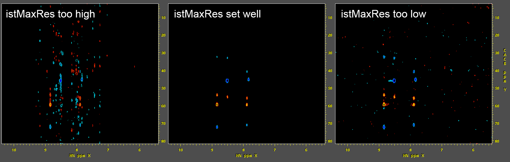

Speed Performance of NMRPipe's IST Reconstruction
The NMRPipe implementation of IST is constructed as an nmrPipe processing script, with the forward and inverse Fourier transform steps performed via the usual nmrPipe pipelines. As a result, it is not particularly fast. That said, it does not require any special computing hardware or large memory, but can still benefit when used on multi-cpu systems. Each iteration of NMRPipe's IST performs the equivalent of three Fourier transforms of the indirect dimensions, and convergence typically requires between 100 to 300 iterations. For example:
CBCANH Uniformly Sampled (512x2)(24x2)(48x2): FT 2 sec FT with Linear Prediction 32 sec IST NUS Zero Fill 300 sec (124 iterations) CBCANH NUS 33% of (512x2)(24x2)(48x2): IST 184 sec (152 iterations) N15-NOE Uniformly Sampled (1202x2)(70x2)(26x2): FT 4 sec FT with Linear Prediction 2 min 30 sec IST NUS Zero Fill 20 min 21 sec (119 iterations) N15-NOE NUS 25% of (1202x2)(70x2)(26x2): IST 9 min 50 sec (257 iterations)
Demo Data for Non-Uniform Sampling (NUS) in NMRPipe
The NMRPipe Demo Data Collection includes NUS examples kindly provided by Robert Brinson and Luke Arbogast at IBBR, Jinfa Ying at the NIH, Prof. Stefano Ciurli at the University of Bologna, and Massimo Lucci at the University of Florence.
There are several possible schemes for organizing NUS data during acquisition, and the schemes used for the demo data here might not be suitable for every type of NUS measurement. And as noted previously, there are many tools available from other labs for reconstructing NUS data, and they will often have schemes for converting NUS data that are different from the ones discussed here.
-
In the demo examples, each individual spectral data directory will have a
script
fid.comto perform conversion steps, and a scriptproc.comto perform processing. -
For the conventional data, there are also scripts "xyz.ist.com" (3D data)
and
ft2.ist.com(2D Data) which demonstrate how to apply the NUS Zero Fill approach using IST as an alternative to Linear Prediction. For comparison, the conventional data will also include Linear Prediction sciptsxyz.lp.comorft2.lp.com. -
Some spectral data directories will have a script
start.comthat illustrates how to start the bruker or varian conversion interface for that particular data, in order to account properly for NUS details. This is for informational purposes only, and thestart.comscripts are not used directly in the demos. -
Data directories will have a script
clean.comwhich deletes all previous results. They may also have a scripttmpClean.comto delete intermediate results. -
Directory:
demo/nus/varian_nus/indanone2d
2D phase-sensitive HC spectra with and without NUS. -
Directory:
demo/nus/varian_nus/mag
2D Magnitude-Mode COSY spectra with and without NUS. Currently, the conversion scripts for Magnitude-mode data are not automatically generated, so these examples use conversion scripts that were created manually. -
Directory:
demo/nus/varian_nus/ubiq3d
3D HN-NOE spectra with and without NUS. -
Directory:
demo/nus/bruker_nus/2d_format
2D phase-sensitive HC spectra with and without NUS. -
Directory:
demo/nus/bruker_nus/br_format
A 3D Example measured with a NUS pulse sequence from Bruker. No corresponding conventional spectrum is included. -
Directory:
demo/nus/bruker_nus/vc_format
3D spectra with and without NUS,measured using pulse sequences from the NIH. The data are recorded in the same format as used in thebr_formatexamples above, so the details of conversion are similar. -
Directory:
demo/nus/bruker_nus/vd_format
Examples measured with and without NUS according to an older "legacy" NUS scheme as implemented according to M. Karra, Ch. Fares, A. Gutmanas, and C.H. Arrowsmith. Spectra in this format require a different initial conversion step compared to the schemes above, and a specific command-line argumentbruker -vdlist ...is needed in order to generate the correct conversion scheme. This particular data also uses NUS schedules which require the option Reverse NUS Column Order - Directory:
demo/nus/varian_nus/indanone2d/indanone_hsqc_std.fid - Directory:
demo/nus/varian_nus/ubiq3d/n15noe_std.fid - Directory:
demo/nus/bruker_nus/2d_format/std - Directory:
demo/nus/bruker_nus/vc_format/13.hnca_full - Directory:
demo/nus/bruker_nus/vd_format/std
Varian/Agilent Format:
In addition, conventional data directories have a script nuszf_demo.com
demontrating the NUS Zero Fill alternative to Linear Prediction. In each
case, the ordinary Fourier transform spectrum will be displayed along with
Linear Prediction and IST results: