|
|
Introduction
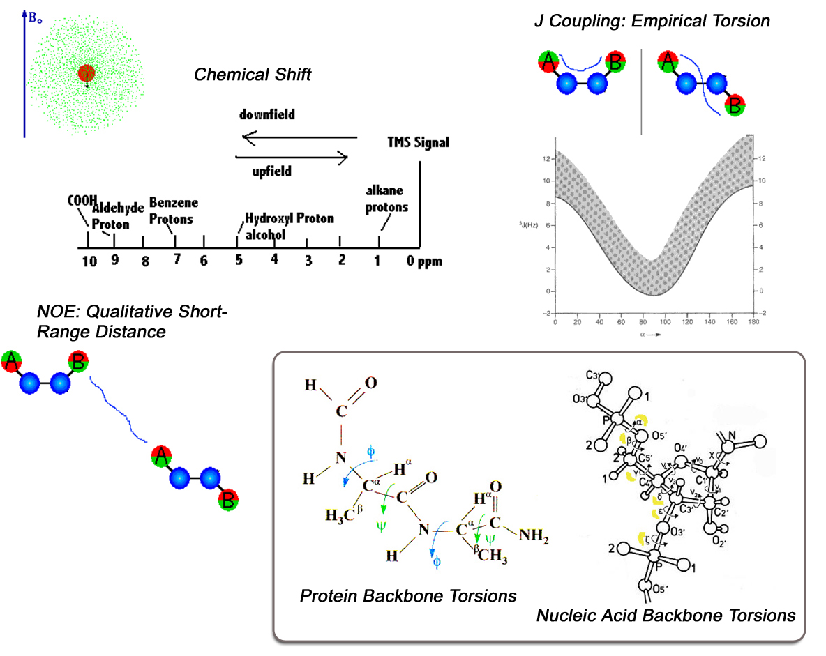
Conventional NMR protein structures are derived from large numbers of short-range
inter-Hydrogen distances extracted from peak heights in NOE spectra. Since quantitative
interpretation of NOE data requires prior knowledge of both the protein structure and its
overall dynamics, NOE distances are generally used in a qualitative way during a typical
structure determination (i.e. classes of short-distance, medium distance, long distance).
These short-range distances are commonly supplemented by J-coupling values, which are
interactions taking place through chemical bonds. Since these interactions generally span
only one, two, or three chemical bonds, they are also short-range in nature. J-couplings
can be measured with great precision. However, they are interpreted on the basis of
empirical calibration curves (Karplus curves) which relate J-coupling values to molecular
torsion angles. So, these relationships are often approximate, and they are commonly
ambiguous, which is to say that a given observed J-coupling might be consistent with two
very different torsion angles.
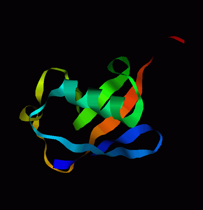
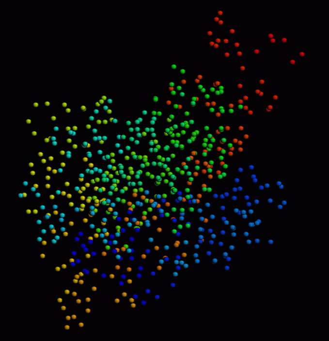
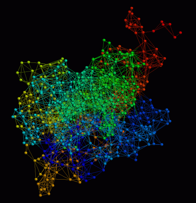
If we consider the complexity of this short-range information, even for a modest protein
fold like the 76-residue ubiquitin, the difficulty of conventional NMR structure
determination becomes apparent. Without counting stereo-specific interactions, or
interactions within residues, the H-atoms in ubiquitin comprise a network of more than 1400 interactions
where nuclei are within 5 angstroms. It is this complicated network which must be
characterized in some way in order to conduct a conventional NMR structure
determination.
So, in order to make NMR structure calculation simpler, we would like to find ways
which do not require analysis of such a complex network of interactions. And, in order to
make NMR structure calculation more precise, we would like to rely primarily on
parameters which can be interpreted quantitatively.
Chemical Shifts
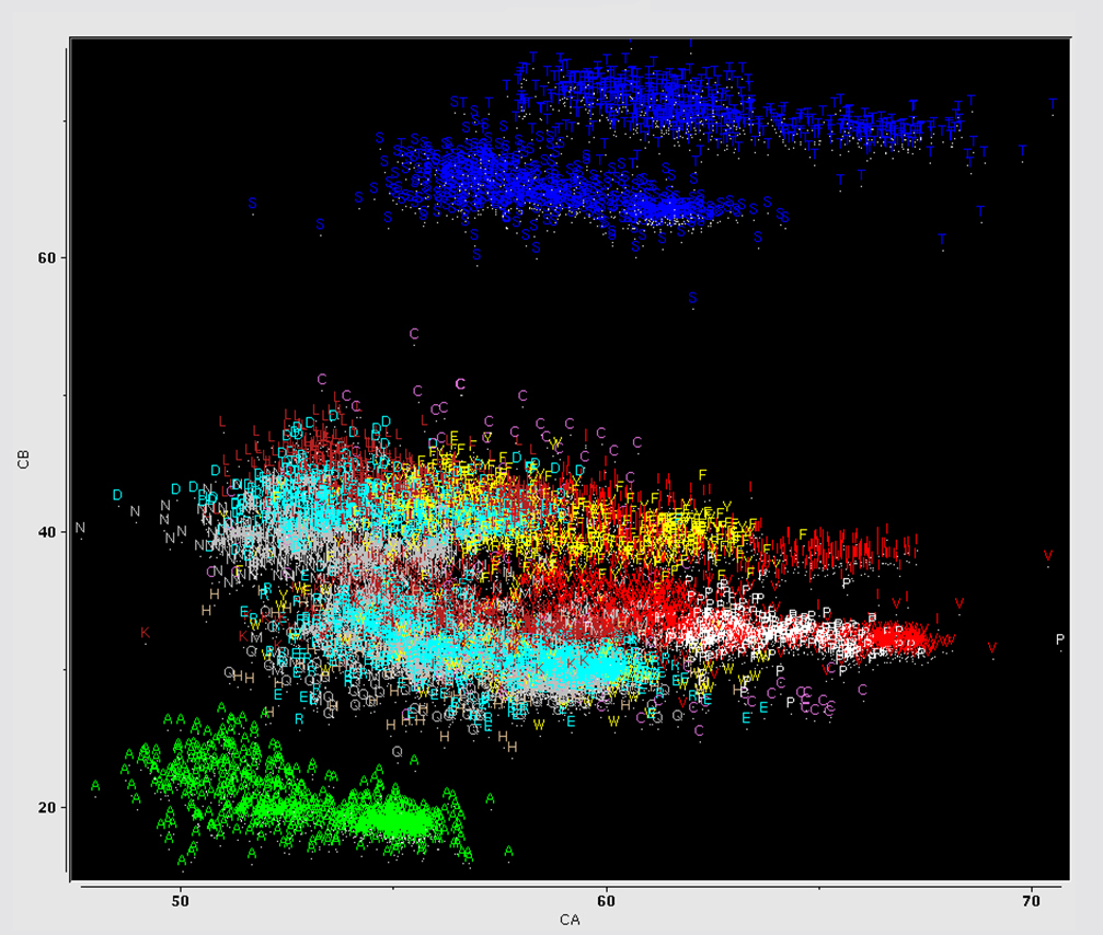
In the first stages of NMR structure determination, we commonly assign the chemical
shifts of the backbone atoms. These chemical shifts are strongly correlated with residue
type, as shown in the plot of C-Alpha vs C-Beta chemical shift values, colorized by amino acid
type. At one extreme lies Ala residues, at the other, Ser and Thr. We can roughly
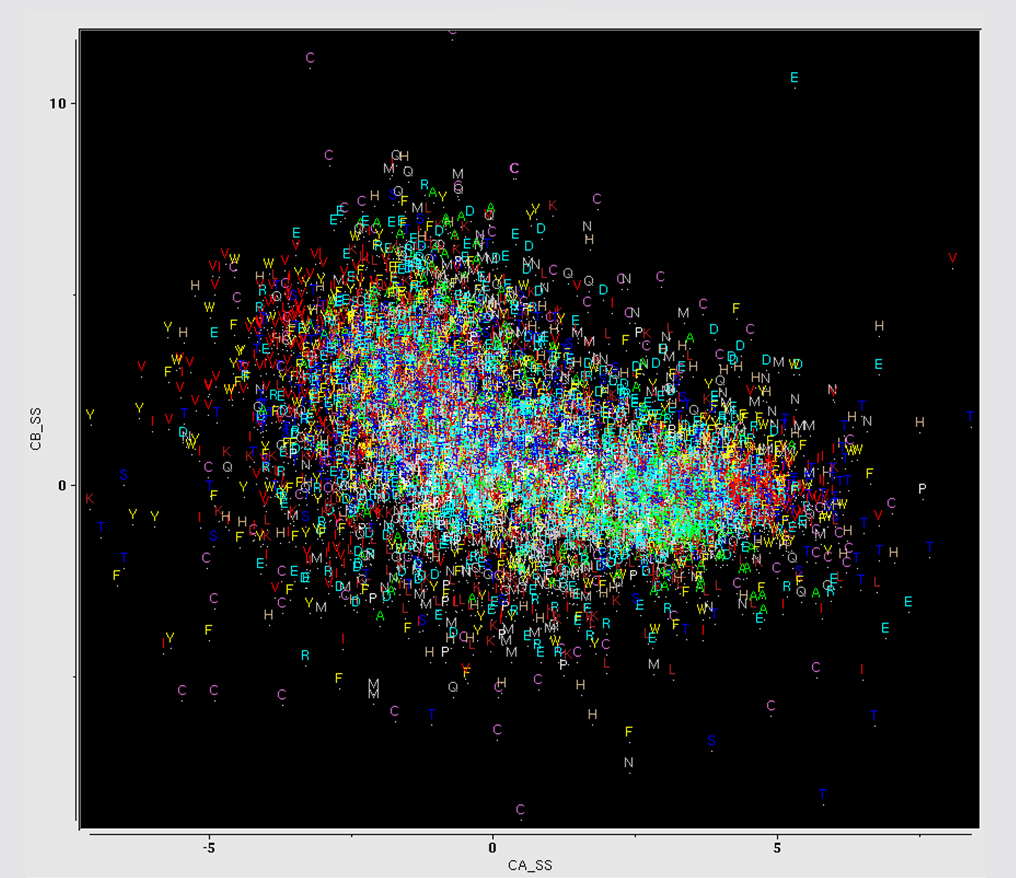
compensate for residue-type differences by subtracting residue-specific
random coil shift values, to generate secondary chemical shifts. An example is shown in this plot of C-Alpha vs C-Beta secondary chemical shift values colorized by residue type. As indicated in the
figure, the secondary shift distribution is roughly similar for all residue types, and is not
random.
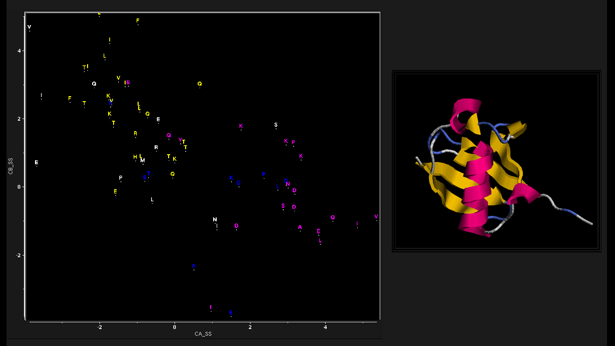
As a clue to the information contained in secondary chemical shifts, consider the plot of C-Alpha vs C-Beta secondary shift for ubiquitin residues, colorized by structural motif.
As shown, secondary shifts from helical residues tend to have values which are different
from secondary shifts of residues in beta-sheets. In other words, the backbone secondary chemical shifts contain information about the backbone structure.
TALOS-N: Prediction of Backbone and Sidechain Angles from Chemical Shifts
In an attempt to exploit this secondary shift information quantitatively, we originally used a simple
database mining approach, implemented in the TALOS system. In this system, we have a
database of known high-resolution structures and their measured chemical shifts. Then,
given secondary chemical shifts of a triplet of residues in an unknown protein, we can
search the database for triplets which have similar secondary shifts. If we find several
good matches in the database, we can assume that the backbone angles of the central
residues in a database triplet will be good predictors for the phi and psi angles in the
unknown protein. In practice we assemble a list of several of the best matches from the
database, which originally contained only 20 high-resolution protein structures.
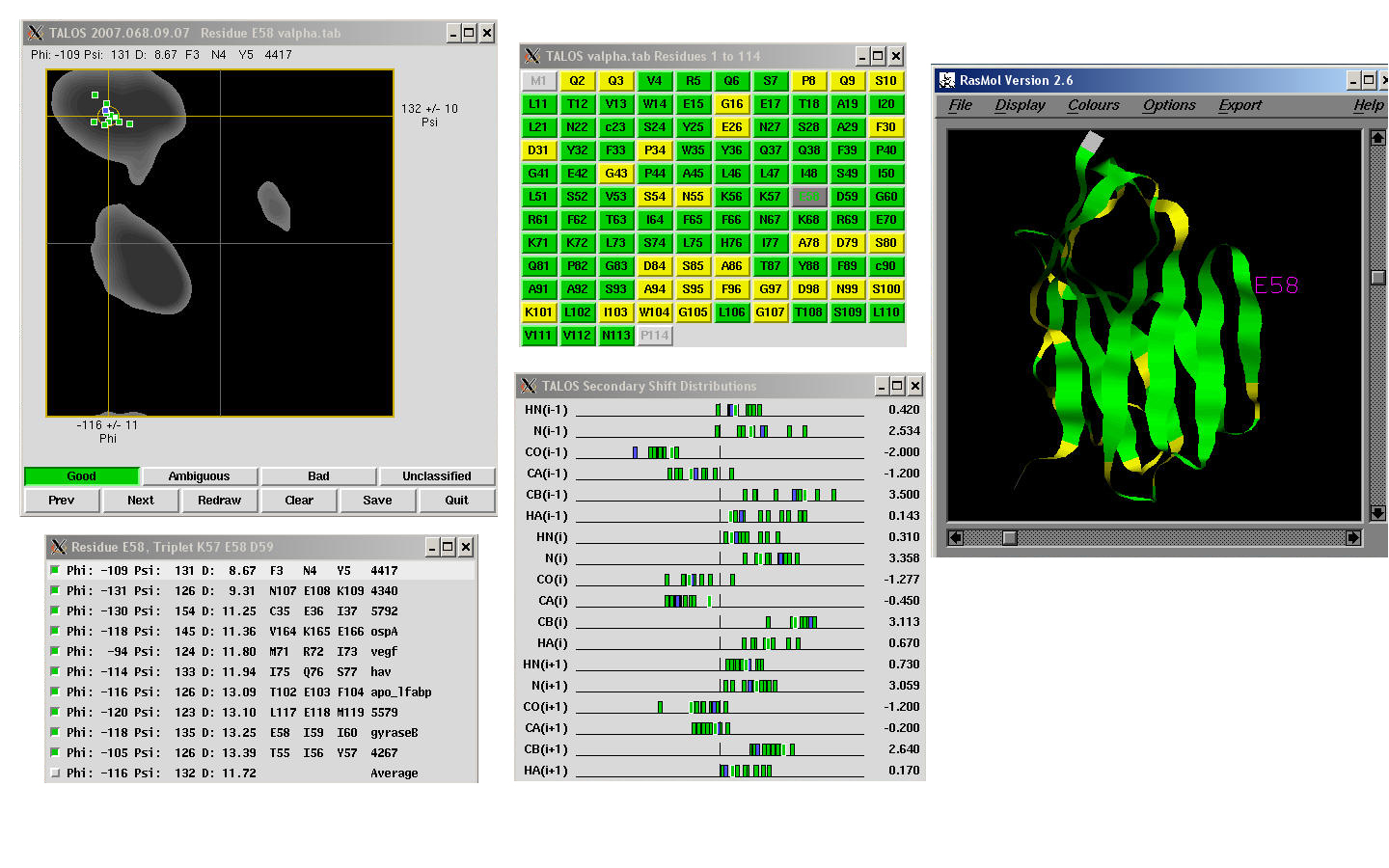
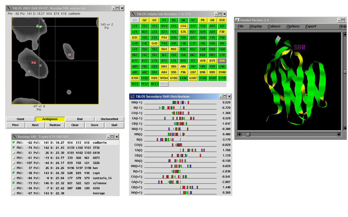
Cross-validation can be used to characterize TALOS by testing how
well each given known protein could be analyzed based on the remaining proteins in the
database. For most residues, there is a clear consensus of phi and psi values
in the best database matches, and in these "good" cases, the average and standard
deviations of the phi and psi angles from the database are used as quantitative predictors
for the backbone angles in the target protein. In the remaining cases, there is no
consensus on phi and psi angles from the closest database matches; these "ambiguous" cases are not used for prediction purposes.
Since the initial development of TALOS, improved versions include a larger database of protein structures,
and the database search is augmented by combining search results with predictions from an Artificial Neural Network.
The latest version, TALOS-N can also make predictions
about sidechain orientation. TALOS-N provides phi and psi estimates to better than 15 degrees RMS, although for
about 3.5% of the TALOS predictions, the predicted angles are substantially different from
the angles found in the reference -X-ray structures. However, a substantial fraction of this 3.5% appears to reflect
genuine differences relative to the crystalline state, and the true error rate therefore is believed to be considerably lower.
TALOS-N can be used via a web-based server:
spin.niddk.nih.gov/bax/nmrserver/talosn.
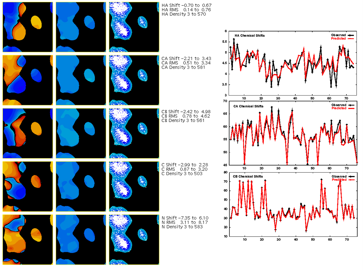
SPARTA+: Prediction of Backbone Chemical Shifts from Protein Structure
Given the information in the TALOS database, it is also possible to estimate backbone
chemical shifts for a proposed structure. The simplest approach uses the database
information to create Ramachandran surfaces of secondary chemical shift distribution with respect to phi and psi. Chemical shifts for a specific phi/psi value can be found
simply by extracting the secondary shift from the given phi/psi point in the surface, and
then adding a suitable random coil value. This simple approach, based on phi/psi values
for individual residues, predicts backbone shifts with accuracies C-Alpha: 1.12ppm, C-Beta: 1.20ppm,
C': 1.29ppm, N: 3.10ppm, HN: 0.67ppm, and H-Alpha: 0.36ppm.
Even better predictions can be performed via the Artifical Neural Network approach used by TALOS-N, as
implemented in the SPARTA+ program. SPARTA+
predicts backbone shifts with accuracies C-alpha: 0.92ppm, C-beta: 1.13ppm, C': 1.07ppm, N: 2.45ppm,
HN: 0.49ppm, and H-alpha: 0.25ppm.
SPARTA+ can also be used via a web-based server: spin.niddk.nih.gov/bax/nmrserver/sparta.
Dipolar Couplings
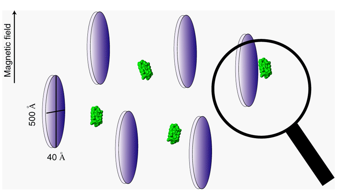
In an isotropically tumbling molecule, dipole-dipole interactions are averaged to zero.
But, if the molecule is in the presence of an aligned medium such as a liquid crystal, the
molecule will interact with the aligned medium, and will no longer tumble isotropically.
Then, dipole-dipole interactions will no longer be averaged to zero, resulting in a dipolar
coupling. These dipolar couplings can generally be measured by the same methods used
to find J-couplings. And, the mathematical form for dipolar couplings can be described
exactly for a rigid molecule, as follows.
|
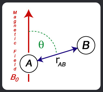
For the purpose of deriving the resonance frequencies (i.e., splittings produced by dipolar coupling) only the z component of the local field of one nuclear dipole at the
position of the second nucleus is relevant (secular approximation). So, for spins of atoms A and B:
Dipolar Splitting Hdd = DABmax< IAz IBz
(3cos2q-1) >
where
the <> brackets refer to the time or ensemble average, which are
equivalent for isotropic and aligned solution,
q is the angle between the A-B internuclear vector and the magnetic
field and:
DABmax= -mo(h/2π)gAgB/(4π2rAB3)
|
|
is the dipolar interaction value, which is the dipolar coupling that would be
observed for the static (completely aligned) molecule.
The constant, -mo,
is the magnetic permittivity of vacuum, h is Planck's constant,
gX is the magnetogyric ratio of
spin X, and rAB is the distance between nuclei A and B.
Some common dipolar interaction values
for protein dipolar couplings are given in the following table. Note that these static couplings are very large; this means
that in practice, a weak alignment of about one part in 103 or 104 will suffice to give rise to
a measurable coupling:
| Atom Pair A - B | Dipolar Interaction Value
DABmax | |
| HN - N | -21,585 Hz | |
| HN - C' | 6,666 Hz | |
| C' - N | -2,609 Hz | |
| HA - CA | 44,539 Hz | |
| C' - CA | 4,285 Hz | |
| CA - CB | 4,150 Hz | |
|
|
The residual
dipolar splitting between spins A and B equals:
DAB = DABmax
< P2(cosq)> with P2(x) =
1/2(3x2 - 1).
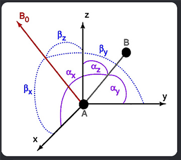
If the molecule is rigid, the orientation
of the internuclear vector, rAB,
in an arbitrary molecular coordinate system can be described by the angles ax, ay,
and az between the vector
and the x, y, and z axis of the coordinate system. The angles bx,
by, and bz define the instantaneous
orientations of each of these axes relative to the static magnetic field. With cosq
being the scalar product between a unit vector in the internuclear direction
and a unit vector parallel to Bo, P2(cosq) can be rewritten as:
<P2(cosq)> = 3/2 < (cosbxcosax + cosbycosay + cosbz cosaz)2
> - 1/2
With Ci = cosbi and ci = cosai, this can be rewritten as:
<P2(cosq)>
=
3/2 [ <Cx>2cx2
+ <Cy>2cy2 + <Cz>2cz2
+ 2<Cx Cy>cxcy + 2<Cx
Cz>cxcz + 2<Cy Cz>cycz
] - 1/2
By writing Sij = 3/2 <Ci Cj>
-
1/2 dij,
where dij is the Kronecker
delta function, we obtain:
<P2(cosq)> =
Si,j={x,y,z}
Sij cosai
cosaj
The 3x3 matrix S is commonly referred to as the Saupe
matrix, the Saupe order matrix, or simply the order matrix. As <Cx>2 +
<Cy>2 + <Cz>2
= 1, the matrix S is traceless, and
with <Ci Cj>
= <Cj Ci>,
S is also symmetric, and therefore
only contains five independent elements.
If the structure of the molecule
is known, then the cosai direction cosine factors can be computed from the atomic coordinates of spins A and B.
This is an important result, because it means that
the five independent elements of the saupe matrix can generally be
solved by linear least squares methods, provided
that dipolar couplings for at least five internuclear vectors are
available. However, if any pair of
internuclear vectors is parallel, and for other special cases such as a set
that includes three mutually orthogonal interactions, more measured couplings
are required. For macromolecules, many
more dipolar couplings are frequently measured, and S is overdetermined.
Its elements are then commonly determined using singular value decomposition.
If the cartesian coordinates of spin A and spin B are {xA, yA, zA} and {xB, yB, zB} we can
define the direction cosines in terms of the coordinates as:
cosax = XAB = (xA - xB)/rAB
cosay = YAB = (yA - yB)/rAB
cosaz = ZAB = (zA - zB)/rAB
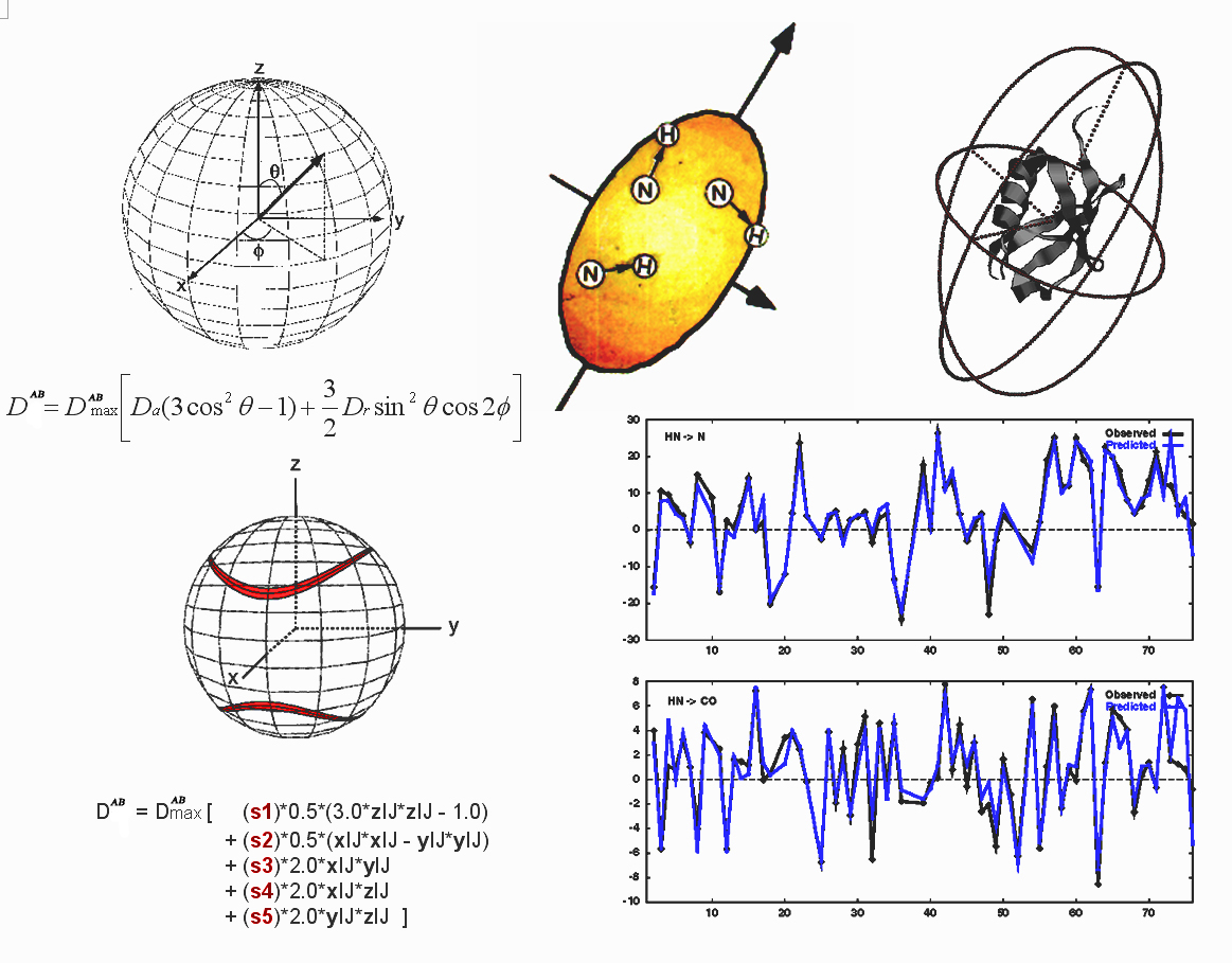
Then, the five coefficients s1 ... s5 can be
determined by SVD using the following basis set:
q1 =
1/2
s-1
|DABmax| (3ZABZAB - 1)
q2 =
1/2
s-1
|DABmax|
(XABXAB - YABYAB)
|
q3 =
2 s-1
|DABmax| XABYAB
q4 =
2 s-1
|DABmax| XABZAB
q5 =
2 s-1
|DABmax| YABZAB
|
where s is the estimated uncertainty
in the measured coupling. The measured dipolar couplings DAB
are used to build a set of equations for solution by SVD:
s-1
DAB = s1q1 + s2q2 + s3q3 + s4q4 + s5q5
Given SVD solutions for coefficients s1 ... s5,
the elements of the order matrix S are:
Sxx = -1/2(s1 - s2)
|
Sxy = Syx = s3
|
Syy = -1/2(s1 + s2)
|
Sxz = Szx = s4
|
Szz = s1
|
Syz = Szy = s5
|
The order matrix is real and
symmetric, and it therefore is always possible to define a molecular axis
system where S becomes diagonal. In a number of applications it can
be advantageous to work in this principal axis frame, where:
DAB(ax,
ay, az) = 3/2
DABmax {[
<Cx>2cx2 + <Cy>2cy2
+ <Cz>2cz2]
- 1}
where
<Ci>2 corresponds to the probability of
finding the i-th axis parallel to the
magnetic field. Only the relative
differences in the <Ci>2 values contribute to the
residual dipolar coupling. So, writing
<Ci>2 = 1/3 + Aii , the
coupling can be expressed in polar coordinates (q
= az; cz = cosq; cx = sinq cosf; cy
= sinq sinf) to yield:
DAB(q,f) = 3/2 DABmax [cos2q Azz + sin2q cos2f Axx + sin2q sin2f Ayy]
Defining |Azz| > |Ayy|
> |Axx|, and using Ayy + Axx = -Azz; 2sin2f = 1 -
cos2f; and 2cos2f = 1 + cos2f,
this can be rewritten as:
DAB(
q,f)
= 3/2 DABmax
[P2(cosq) Azz
+ 1/2sin2q
cos2f (Axx - Ayy)]
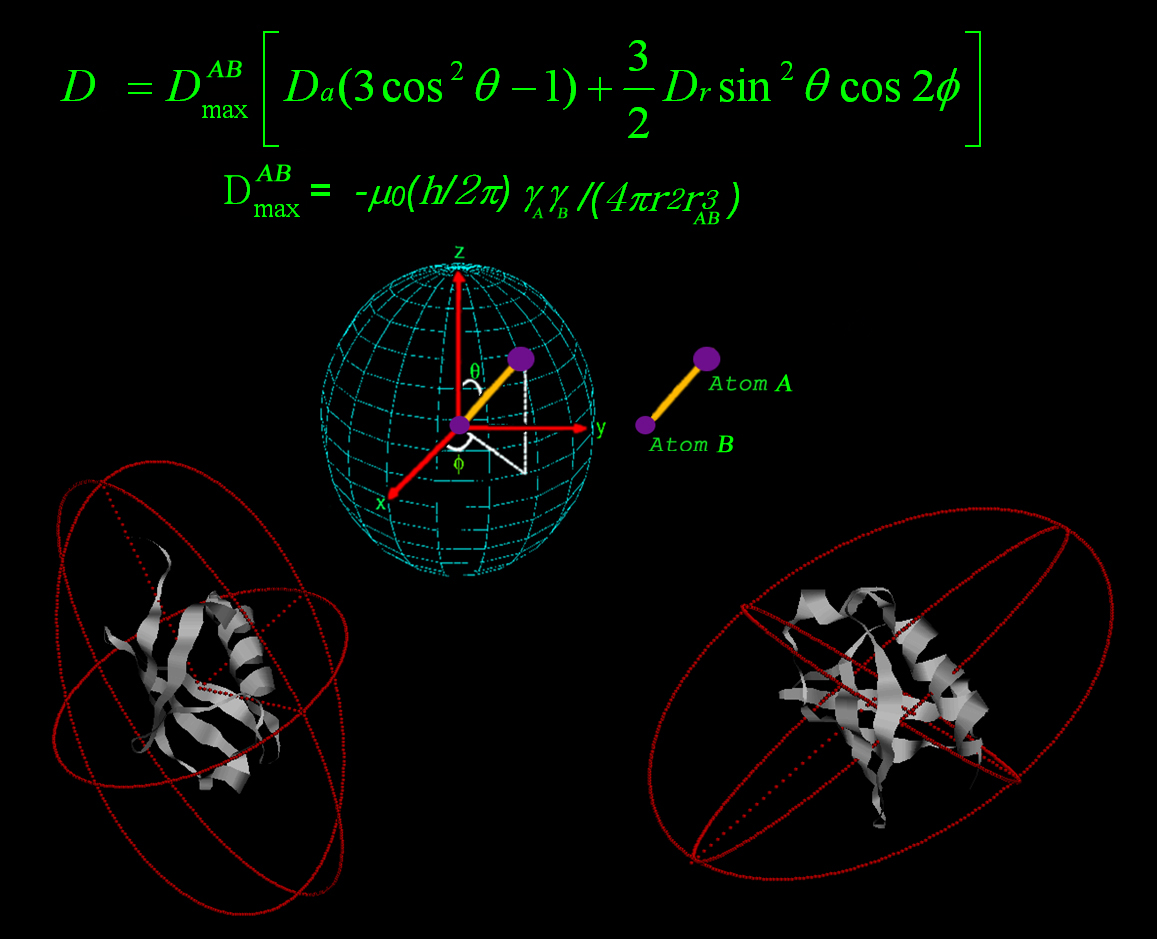
This leads to an expression of dipolar couplings in terms of alignment tensor parameters. From a graphical point of view,
the alignment tensor can be visualized in terms of a 3D ellipsoid whose orientation corresponds with the axes of alignment, with the dimensions of
the ellipsoid along each axis being Azz, Ayy, and Axx. As noted above, by definition Azz is the longest axis,
Ayy the next longest, and Axx the smallest.
Defining an axial component of
the alignment tensor Aa = 3/2Azz,
and a rhombic component, Ar = (Axx - Ayy), results in:
DAB(q,f)
= DABmax [P2(cosq) Aa + 3/4
Ar sin2q cos2f]
Note that the maximum value for
<Ci>2 is one, i.e., the maximum for Azz
equals 2/3, and the maximum value for Aa
becomes one when the z axis of the
principal alignment tensor becomes fully aligned with the static field.
The above expression is often rewritten as:
DAB(q,f)
= DABa [(3cos2q - 1) + 3/2 R sin2q cos2f]
where DABa = 1/2DABmax is referred
to as the magnitude of the dipolar coupling tensor, which describes how strongly aligned the molecular system is, and R
= Ar/Aa is the rhombicity, which is the departure of alignment from axial symmetry.
When the molecular system has been rotated so that its coordinate axes
correspond with the alignment tensor axes, then the dipolar coupling can
be computed as follows (this is the form used for our fitting of
dipolar couplings by non-linear least squares, for cases where there
are restraints on one or more tensor parameters):
DAB
= |DABmax| [Daxial (3ZABZAB - 1) + 3/2 Drhomb (XABXAB - YABYAB)]
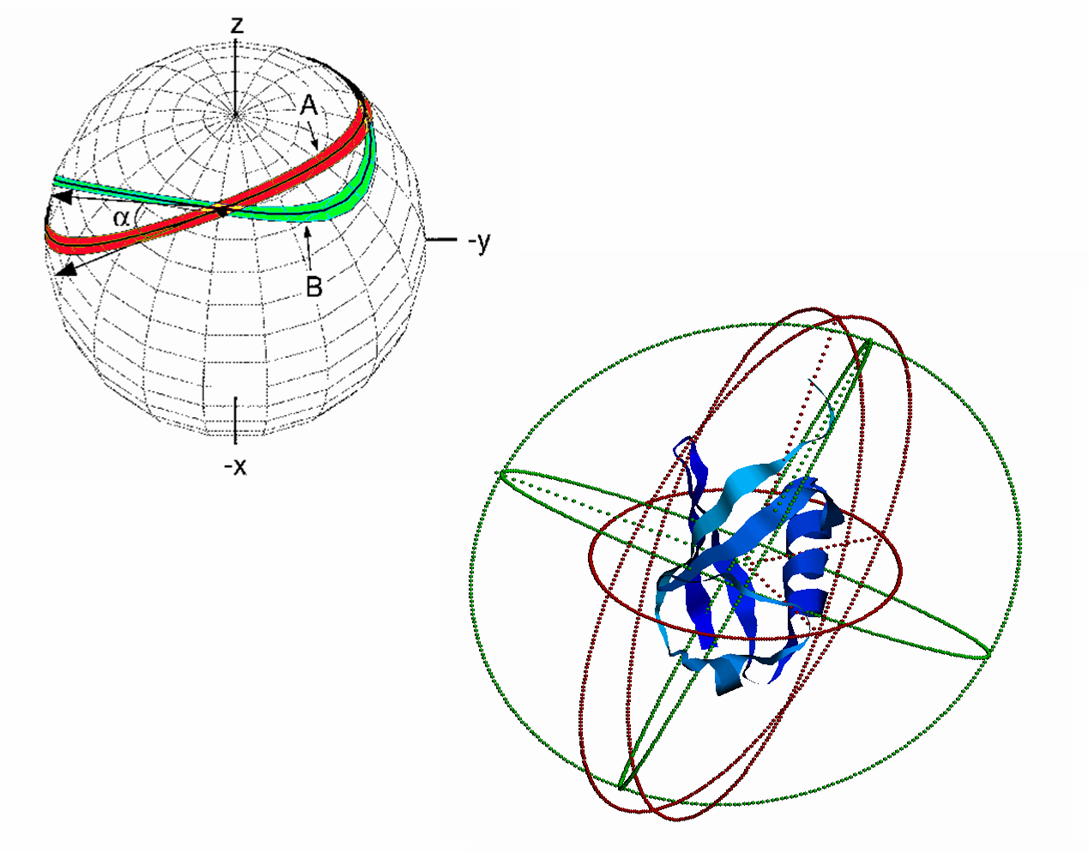
A critical aspect of the dipolar
couplings is their dependence on cos2q,
which in practice means that there are two continuous ranges of
orientation for the internuclear coupling vector which are consistent with a
given coupling value, and they are mirror images of each other. A simple way to reduce this ambiguity is to
prepare two different types of aligned media, for example a neutral one,
and a charged one. The nature of interaction between the target molecular
and the alignment media will be different in the two cases, resulting in
two different and independent alignment systems.
This restricts the orientations to only those positions which are consistent with both alignment tensors simultaneously. Then, only the intersecting orientations will be consistent with
coupling values from both samples.
However, there will still generally be cases that more than one conformation
is consistent with the dipolar data.
Within the context of a protein, residues
are arranged in preferred orientations relative to each other, and in most
cases, only one of these will be consistent with the collection of dipolar
couplings. So, one way to reduce the impact of ambiguity is to only consider
physically realistic protein conformations.
To help resolve potential ambiguity still further, we can employ secondary
structure information from chemical shifts.
The molecular alignment frame serves as a reference system which establishes
the relative orientation of one internuclear coupling vector with respect to
any other, regardless of how far apart these internuclear vectors may be. For example, in the case of
HN-N couplings, dipolar couplings tell about the orientation of an HN-N bond vector
relative to any other HN-N bond vector. This long-range orientational information is
very different in nature from the short-range distance and torsion information
traditionally used in NMR structure calculation, and as we will show, it is a powerful
complement to short-range data.
Direct Applications of Dipolar Couplings
As already explained, dipolar coupling values are determined by orientation. So, dipolar
couplings for two parallel bond vectors should be identical, given scaling factors to
compensate for bond distance and magnetogyric ratios. This can form the basis for some
useful analysis. For example, side chain orientation can be estimated by testing how
dipolar couplings in the sidechain are correlated to parallel bonds in the backbone.
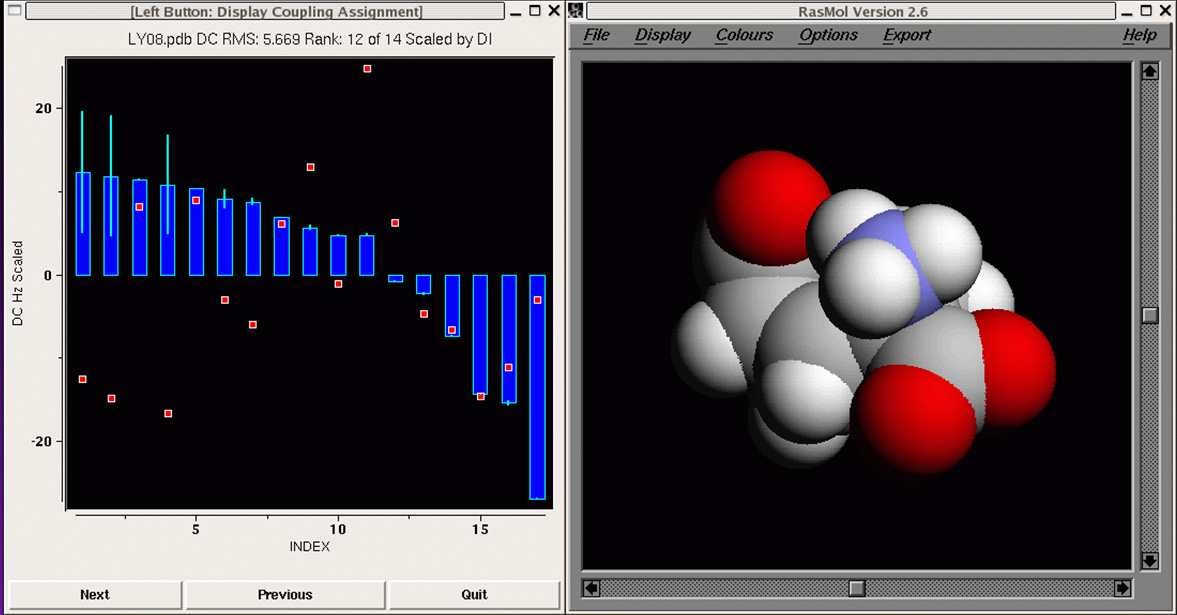
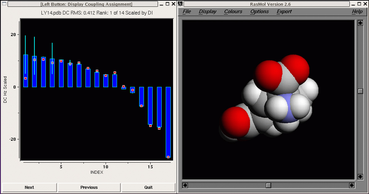
Similarly, relative stereochemistry for molecules with several stereochemical centers can
be identified by testing agreement of observed vs calculated dipolar couplings
for all possible stereoisomers, and finding the stereoisomer with the best agreement
between observed and calculated dipolar couplings.
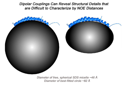
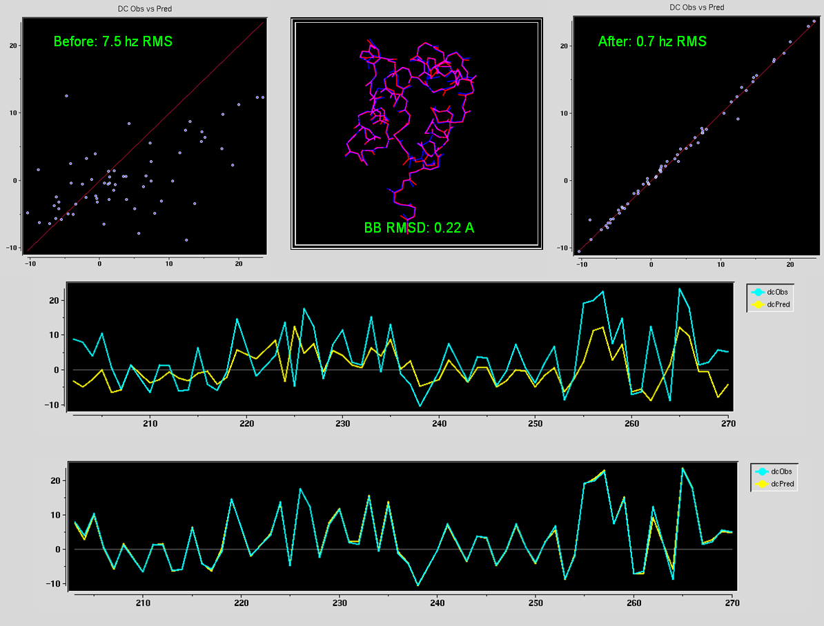
Dipolar couplings can be extremely sensitive to small changes in molecular coordinates, and they can be used directly in conventional structure determination.
For example, consider the initial structure of a 69-residue protein fragment which has a
~7 Hz RMSD between observed and calculated HN-N dipolar couplings. This structure
can be refined by conventional simulated annealing so that the couplings match to better than 1 Hz RMSD, but the refined backbone
structure differs by less than 0.3 angstroms RMSD from the initial structure. As such,
dipolar couplings can reveal structural details which might be difficult to characterize
with NOE distances alone, for example the curvature of an isolated helix, as in the case of
micelle-bound alpha-synuclein.
Structure Determination from Dipolar Couplings as the Primary Data
As noted above, a critical aspect of the dipolar couplings is their dependence on
cos2q which in practice means that there are two continuous ranges of orientation for the
internuclear coupling vector which are consistent with a given coupling value, and they
are mirror images of each other. As also noted, a simple way to reduce this ambiguity is
to introduce couplings measured at another alignment tensor, which restricts the
orientations to only those positions which are consistent with both alignment tensors
simultaneously. Then, only the intersecting orientations will be consistent with coupling
values from both samples. This greatly reduces the ambiguity of dipolar couplings, but does not eliminate it.
It can be noted that bond vectors in a protein are not oriented randomly or uniformly. For
example HN-N bond vector orientation surfaces for ubiquitin and DinI proteins show that
the distributions are systematic, and also different for the two proteins. This argues that when analyzing data for a sequence of many residues simultaneously,
it is not strictly necessary to consider every possible orientation of individual bond vectors when
exploiting dipolar couplings for protein structure determination.
Since protein residues are arranged in preferred orientations relative to
each other, one way to reduce the impact of ambiguity is to
consider only physically realistic protein conformations.
And, to help resolve potential ambiguity still further, we can employ
structure information from other NMR observables such as chemical shifts
in combination with dipolar coupling data. This leads to the database
mining approach called Molecular Fragment Replacement (MFR).
Molecular Fragment Replacement (MFR)
The central concept of MFR is straightforward; identify short fragments of
known high-resolution protein structures whose simulated NMR
parameters are a good match for the observed NMR parameters of
the target protein.
Then, use suitable methods to assemble these fragments into
larger elements of protein structure.
The NMR parameters can include any combination of chemical shifts,
dipolar couplings, J-couplings, sequential NOEs, etc, as well
as residue-type homology. For each individual parameter, such as chemical
shift, a score is computed on the basis of the RMS differences
between observed and predicted values. A linear combination of these
individual scores is used to form an overall MFR score which
is used to rank the fragments.
In practice, MFR uses fragment sizes
of 5-10 residues, currently drawn from a subset of roughly 850 structures
in the
PDB database, all with resolutions better than 2.4 angstroms. This provides
a collection of more than 180,000 fragments, which is large enough
to ensure that all physically realistic short fragment structures are
represented. This means that MFR database mining can be still
be applied to novel proteins which have no known homologous structure
in the PDB.
Our first proof-of-concept result is shown in
the MFR search results for
residues 1-16 of ubiquitin, where we tallied the three best
matching fragments in terms of simulated versus measured chemical
shifts and dipolar couplings. Dipolar couplings for HN-N,
HN-C', N-C', and HA-CA measured in two alignment media were employed.
Using this data in an MFR search, the three database fragments with the
best MFR scores all match the backbone structure of ubiquitin to better
than 1 angstrom RMSD.
In a typical MFR search, we find overlapping collections of fragments
which are best matches (i.e. lowest scores) according to the MFR scoring
procedure.
So for example, using a 7-residue fragment size, an MFR search will identify
the 10 database fragments which are the best match
for residues 1-7 in the target protein, the 10 best matches for residues
2-8 in the target protein, etc.
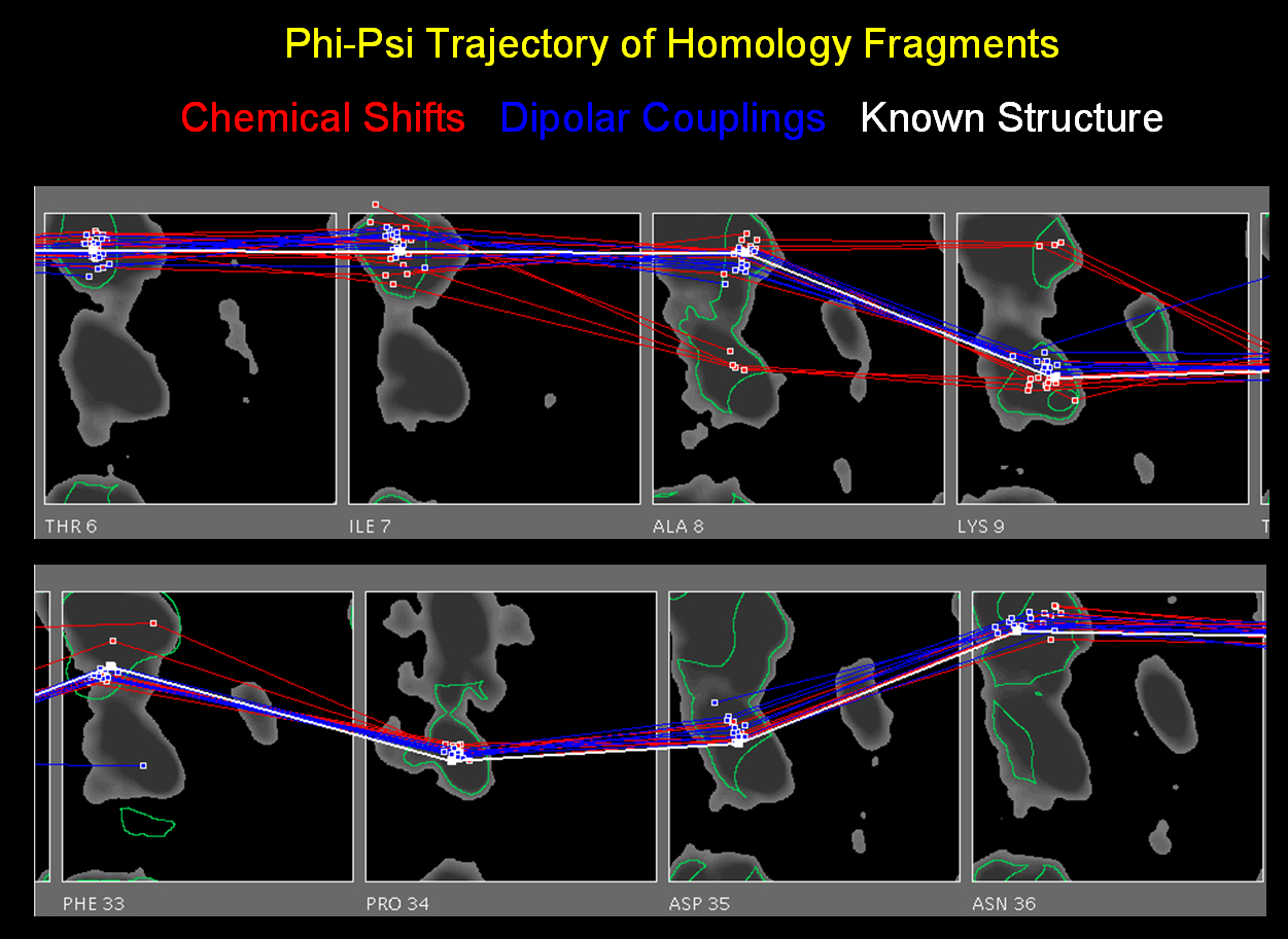
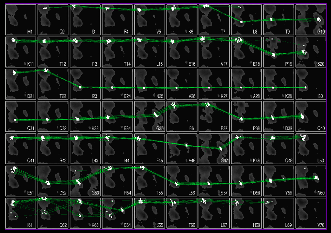
Such a collection of fragments can be visualized as a Ramachandran trajectory where each fragment is represented
as a collection of vectors connecting that fragment's phi,psi backbone angles
on a series of ramachandran surfaces for the target residue sequence.
The ramachandran trajectory of MFR
database fragments for ubiquitin is a good illustration of typical MFR results
where chemical shifts are used in combination with dipolar couplings from
two aligned media. In such results, there are two notable aspects.
First, for the majority of residues where measured NMR parameters are
available, MFR provides unambiguous indication
of the phi,psi conformation. Second, even in regions where the MFR results
show structural diversity, there are generally always some fragments which
are good representatives of the ideal structure. This argues that the
MFR search results should be a powerful and effective precursor to
structure determination, given suitable protocols for converting MFR
results into complete structures.
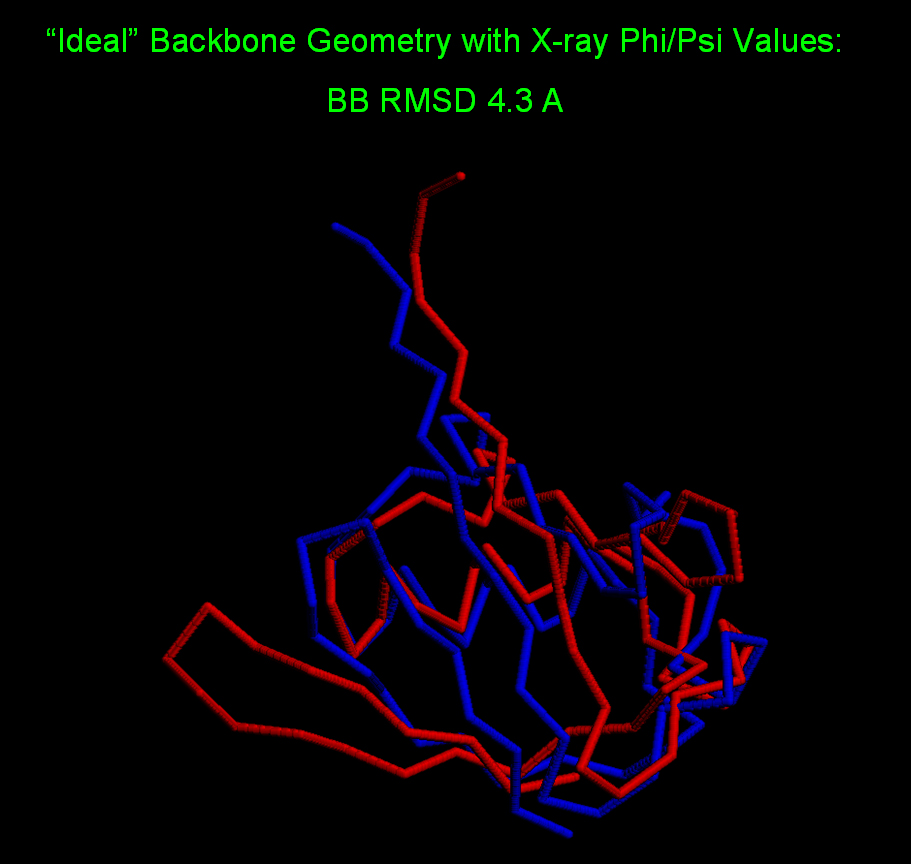
However, it must be noted that it is not easy to use phi,psi conformations
directly to build an entire protein structure. For example,
if the exact phi,psi backbone angles from the crystal structure of ubiquitin
are superimposed onto an ideal planar protein backbone geometry,
the new structure differs from the original by more than 4 angstroms RMS.
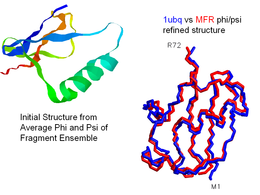
Nevertheless, it is possible to use MFR phi,psi values directly to build
and refine elements of structure from 10 to 50 amino acids long, without
the use of any distance restraints. In the ideal case of ubiquitin,
where 4 types of high-quality dipolar couplings are available in two media
for almost all residues, the entire protein fold can be determined from dipolar couplings and chemical
shifts alone, to a backbone RMS of better than 1 angstrom.
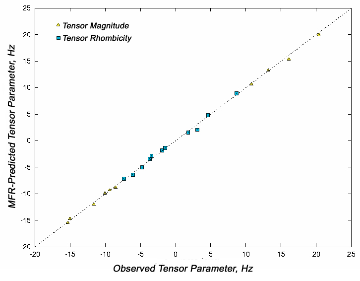
MFR Alignment Tensor Estimates without Prior Knowledge of Structure
As noted above, most of the fragments from an MFR search are good
representatives of the ideal structure of the target.
This means that the tensor magnitude and rhombicity estimates from the best MFR fragments should be good estimates for the alignment tensor parameters of the entire intact protein. These estimates
can be used in later structure refinement steps.
The predicted tensor parameters for the protein as a whole are
calculated from a weighted average of the tensor parameters from
the entire collection of MFR fragments.
The weighting is performed according to the structural consensus
over each given range of residues.
This method can estimate
tensor magnitudes and rhombicities to 0.5 Hz relative to an HN-N coupling.
In the case where two alignment media are available, the MFR results can
likewise be used to compute the relative difference in orientation
between the two tensors, which can also be used as a restraint for later
structure refinement.
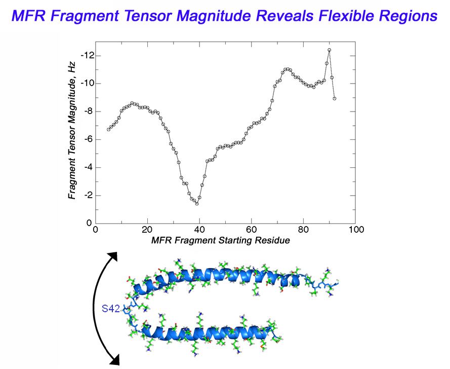
Dynamics Information from MFR
In the case of a flexible backbone structure, the local tensor magnitude is
scaled down by the internal dynamics order parameter. So, a simple plot of
MFR fragment tensor magnitude estimates versus fragment starting residue will reveal the location of flexible regions
as places in the graph where the tensor magnitude drops.
This same approach can also be used to identify cases where domains
within a protein have different alignment tensors.
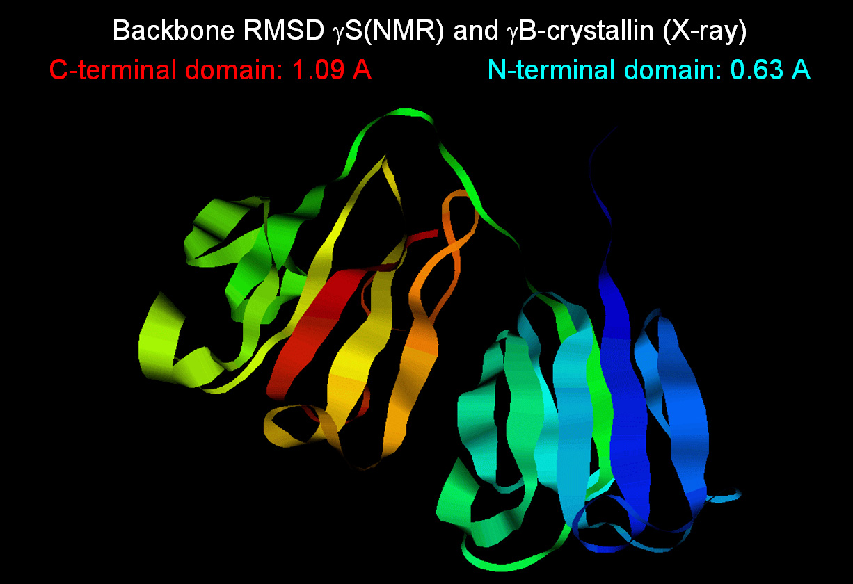
Gamma-S Crystallin: A Practical Application of MFR
The MFR application of Gamma-S crystallin serves as
an example of practical, high-quality structure determination based primarily
on orientational restraints, supplemented by relatively small numbers
of easy-to-assign NOE distances.
Gamma-S is 177 residue protein with two similar domains, for which
a homologous structure (Gamma-B) with 50% sequence identity is known.
Dipolar coupling data in two media were measured. In one medium,
measurements included 144 HN-N, 111 CA-CB, 150 CA-C', and 134 N-C'
dipolar couplings. In the second medium, measurements included
147 HN-N, 135 CA-CB, 153 CA-C', and 139 N-C' dipolar couplings.
Conformational exchange resulted in missing amide signals
for one residue in the N-terminal domain, and nine residues in
the C-terminal domain, so that most of the "missing" coupling data
is associated with the C-terminal domain.
Side-chain c1 angles were
estimated from from
3JNCg and
3JC'Cg couplings, and
c2 angles from 3JCgCd.
A deuterated sample was used to obtain 179 Amide-Amide NOEs, however none
of these represented inter-domain contacts. So, a Gamma-S sample with 13C
labeling for methyl sidechains only was used to obtain 70 Methyl-Methyl NOEs,
and these included 6 inter-domain distances.
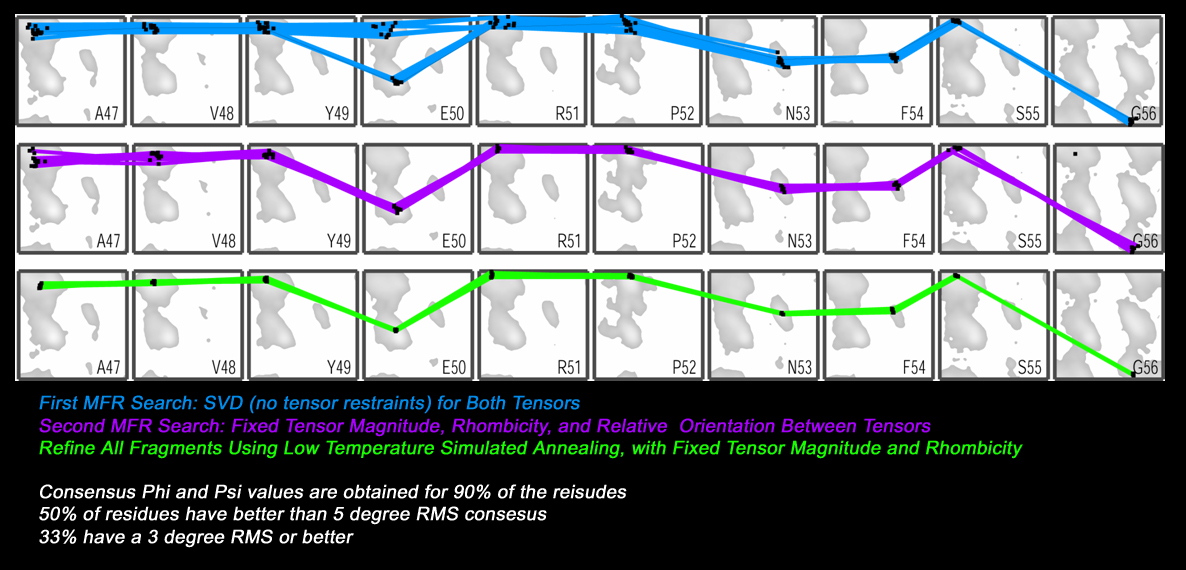
Using this data, the MFR search was
conducted in two stages followed by a fragment refinement step.
In the first MFR search, dipolar couplings were fit to database
fragments using SVD, which is the default approach, and computationally
fast. In this case, the tensor magnitudes and rhombicities are allowed
to assume any value.
So, in some cases, fragments with a "non-ideal" shape can be made to
match the measured dipolar couplings by using tensor parameters
which are not truly representative of the target protein.
To improve this situation, the results of the first MFR search are
using to estimate reasonable tensor magnitude and rhombicity for the
two alignment media. Then, a second MFR search is performed, this
time with the tensor parameters held fixed at the estimated values.
This requires use of non-linear least-squares fitting of the dipolar
couplings, which is much slower. However, this second search with
restrained tensor parameters leads to a collection of fragments with
fewer ambiguities. Finally, the fragments identified by this second
MFR search are subject to conventional low-temperature simulated
annealing refinement, to make small adjustments in the fragments which
improve their overall agreement with the measured dipolar couplings.
In the case of Gamma-S, the resultant collection of refined fragments
has unambiguous phi,psi conformations for 90% of the residues.
Furthermore, these fragments have a high amount of structural consensus,
such that 50% of the residues have better than 5 degree RMS phi,psi
consensus, and 33% of the residues have better than 3 degree RMS
phi,psi consensus.
At this point, we have a collection of structural data which is
more or less ideal for 90% of the residues, but we don't know
in advance which residues are the "ideal" ones. We can use a simple
modification of a traditional annealing scheme to employ this data.
First, all residues the MFR results are converted into phi,psi restraints
for all residues where there is a consensus phi,psi conformation
in all refined fragments. Then, these restraints are used in a conventional
simulated annealing protocol,
along with NOE distances, and the original
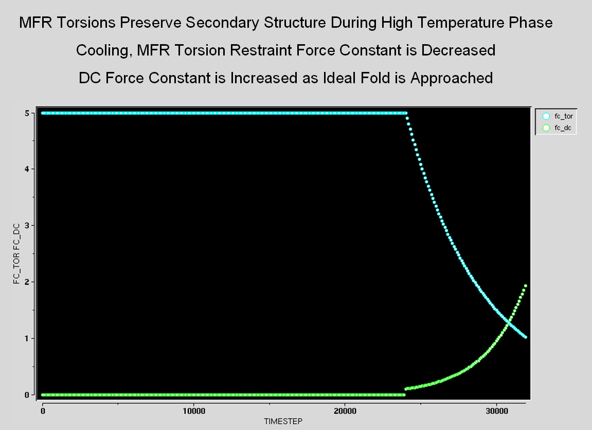
dipolar couplings themselves. In the high-temperature phase,
the force constants for the MFR-derived torsion restraints are held
high, so that the MFR results maintain the local structure at
early stages of the structure calculation.
During cooling, the force constant of the MFR torsions is reduced,
while the force
constant for the NOEs and individual dipolar couplings is increased.
So, as the structure approaches its ideal fold, the MFR torsion
restraints become less important, and the individual dipolar
couplings become more important in maintaining the local structure.
This allows the final structure a chance to overcome any incorrect
conformations in the MFR torsion restraints. In this case, the final MFR-derived structure of Gamma-S agrees with its homolog Gamma-B to
0.63 angstroms RMS for the N-terminal domain backbone, and 1.09
angstroms for the C-terminal domain. In particular, the N-terminal
agreement is among the best between any NMR structure and homolog.
Summary
Dipolar couplings and MFR database mining form the basis for a
new approach to structure determination based primarily on
quantitative orientational restraints, supplemented by
small numbers of NOE distances. The MFR approach can also be used
to estimate tensor parameters without prior knowledge of the
structure, and to probe the dynamics of the molecular system.
In our applications so far, the MFR approach has been quicker
than conventional NMR structure
determination, and has yielded better quality structures.
It has also provided structural information for systems where NOE
data is not obtainable or is not revealing.
|